Calculating coefficients for Affine Transformation

Introduction

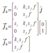
Geospatial rasters inherently have two coordinate systems associated with them: pixel indices (i,j) and real world coordinates (x,y). For the simple case covered on this page, where a linear transform is sufficient to relate the two coordinate systems, physically significant parameters may be used to define the linear relation. These physically significant parameters control the magnitude and orientation of the basis vectors i_b and j_b defined in the following figure:

In the above image, the x and y axes represent geocoordinates (e.g., easting and northing in a projected system or longitude and latitude in a geographic system.) The basis vectors i_b and j_b are the transformed unit vectors i and j, respectively. The magnitude of the basis vectors represent the distance between grid cells in the units of the geocoordinate system. The angle between the x axis and basis vector i_b is given by θ_i. The angle between the two basis vectors is designated by θ_ij. In a "normal" right handed coordinate system, θ_ij is +90 degrees, but the value -90 degrees (indicating that the j axis needs to be flipped) is also very common. Any value other than plus or minus 90 degrees indicates that the linear transform includes shearing parallel to the i axis.

These simple linear relationships between pixel coordinates and geocoordinates are typically represented as modular combinations of individual transformations. Regardless of the order in which they are combined, a linear transform results. The transform is then used to convert coordinates between the two coordinate systems of the raster. This page describes a set of ubiquitous individual transformations and combines them to produce a specific transformation which respects the physically significant parameters which a typical user is likely to be interested in.

The physically significant inputs which drive the model are:

• The magnitude of the i_b basis vector (distance between pixels along i axis)
• The magnitude of the j_b basis vector (distance between pixels along j axis)
• The angle θ_i (the angle by which the raster's grid needs to be rotated, positive clockwise — for compatibility with "heading/bearing")
• The angle θ_ij (the angle from the i basis vector to the j basis vector positive counterclockwise — for consistency with right-handed coordinate system)

The level of math required to follow along is advanced high school algebra or introductory college algebra. It should be accessible to anyone with a science, math, or engineering background. Lacking this, the nontechnical introduction to ​matrix multiplication on wikipedia should provide sufficient background.

Individual operations

This page discusses operations in two dimensions only. Each operation is presented as a 2x2 matrix, and each operation performs only one function. These operations were taken from ​wikipedia. While the matrices presented here contain the bulk of the functionality of a finished affine transform, they are not complete affine transforms themselves. Each transformation will be presented in matrix and equation form: they are equivalent representations.

Rotation

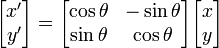
There are two directions one can rotate in two dimensions: clockwise and counter clockwise. The transformations are different. The counter-clockwise rotation is:

• x' = xcosθ − ysinθ
• y' = xsinθ + ycosθ

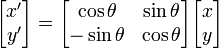
To rotate in the clockwise direction:

• x' = xcosθ + ysinθ
• y' = − xsinθ + ycosθ

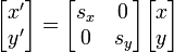
Scaling

Scaling is used to set the size of the raster's grid cells in the x and y direction. The transformation is as follows:

• x' = x s_x
• y' = y s_y

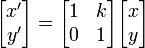
Shearing

Shearing is visually equivalent to a "slanting" which is parallel to either the x or the y axis. This is a less common operation than rotation and scaling. These are presented as individual operations: one for each axis.

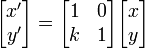
Shearing parallel to the x axis takes the following form.

• x' = x + k_xy
• y' = y

While shearing parallel to the y axis has this form:

• x' = x
• y' = k_yx + y

Reflection

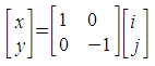
Reflection across the x axis (or "flipping" the y axis) is accomplished with the following transform:

• x' = x
• y' = -y

Combining individual operations

Whenever more than one of the above operations is required, they may be combined using ​matrix multiplication. As an example, all of the above matrices will be combined into one. The result of such a combination is still not an affine transform, however. It is just a 2x2 matrix which has all the individual transformation functions aggregated into it.

We will be calculating a new matrix, O, which is the aggregate of the following individual operations:

1. Reflection across the i axis
2. Scaling along the i and j axes
3. Shearing parallel to the i axis
4. clockwise rotation around the origin (by θ_i)

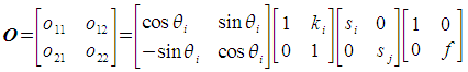
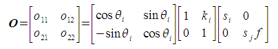
We do this by multiplying the 2x2 matrices of the individual operations together, as follows:

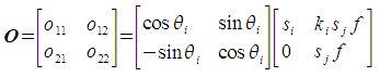
We will perform the matrix multiplications on the right hand side one at a time.

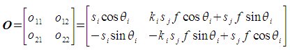
The above matrix equation is shorthand for four equations: one equation each for o₁₁, o₁₂, o₂₁ and o₂₂.

• o₁₁ = s_i cos(θ_i)
• o₁₂ = k_i s_j f cos(θ_i) + s_j f sin(θ_i)
• o₂₁ = -s_i sin(θ_i)
• o₂₂ = -k_i s_j f sin(θ_i) + s_j f cos(θ_i)

Notice that none of the coefficients in the O matrix may be said to represent pure scaling, rotation or shearing. Rather, they all have components of each of these operations factored in. The final matrix equation has some terms which need to be calculated. This will be performed in the next section using the real input parameters. Once these terms have been calculated, they may be plugged into the above equations to arrive at the coefficients which must be stored in the geotransform matrix.

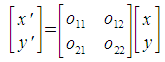
Also notice that it is not necessary to compute this matrix every time one wants to convert between pixel indices and geographic location. The coefficients are computed once for the entire raster, and may be reused for every pixel calculation. You would use this aggregate matrix O exactly as you would use any of the individual matrices:

• x' = o₁₁ i + o₁₂ j
• y' = o₂₁ i + o₂₂ j

Calculating terms

The linear transform matrix O, calculated in the previous section, contained some terms which need to be calculated from the provided, physically significant inputs. These terms are s_i, s_j, k_i and f.

Reflection term

The coefficient f essentially represents a decision as to whether the j axis needs to be flipped. If f=1, the j axis is not flipped. If f=-1, the j axis is flipped. The decision of whether to flip the j axis is controlled by the θ_ij input parameter as follows:

• if θ_ij < 0 then f = -1
• if θ_ij ≥ 0 then f = 1

Scaling along i axis

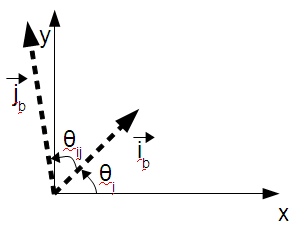
Scaling along the i axis is represented by the s_i term. We will set it using the magnitude of the i_b basis vector. This section will go about proving that this is a valid thing to do.

To simplify things and remove clutter from the equation, note that the final component of the aggregate transform (rotation) does not affect the magnitude of the basis vector. So, the i unit vector projected thru a non-rotating transform is calculated as follows:

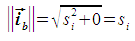
The magnitude of i_b is given as follows:

From the above:

• s_i = magnitude of i_b

Shearing parallel to i axis

Any value of θ_ij which is not plus or minus 90 degrees indicates that shearing parallel to the i axis is required. This produces diamond shaped (non-rectangular) pixels in the output. In this section, we calculate a value for k_i from the provided value for θ_ij. Note that since the rotation of the entire grid does not affect the angle between the two basis vectors (because they are both rotated by the same amount), we solve for k_i in the non-rotated system.

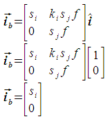
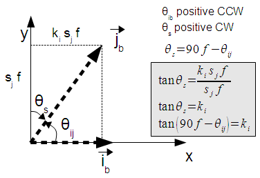
The j_b basis vector is represented as follows:

Illustrated, the j_b basis vector looks like this:

In this diagram, θ_s represents the shearing angle, which is a ​complementary angle to θ_ij. The provided equation defines θ_s = 90f - θ_ij in order to have a single equation which is correct whether the j axis is flipped or not.

• k_i = tan(90f - θ_ij)

This equation passes the basic sanity check that k_i=0 when θ_ij is plus or minus 90 and f is defined as above. Note that θ_ij = 0 or 180 degrees is an error. This is not just a mathematical artifact. The basis vectors are not allowed to be parallel to each other because then you no longer have a grid.

Scaling along the j axis

Scaling along the j axis is represented by the s_j term. We will set it using the magnitude of the j_b basis vector and the above defined terms. This will be more complex than the corresponding calculation for the i axis, due to the possible presence of shearing.

The j_b basis vector is represented as follows:

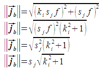
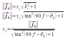
The magnitude of j_b is then calculated as follows:

Substituting for k_i and solving for s_j:

Constructing the affine transformation

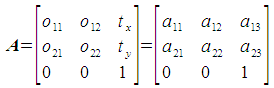
The 2x2 matrix O is the upper-left hand corner of the affine transformation, which is the 3x3 matrix, A. The right hand column contains the offsets, or translation, of the raster in the x and y directions. The bottom row is always filled with the numbers 0, 0, 1. The result of this is that there are six parameters to an affine transformation which can actually change, as shown:

• a₁₁ = o₁₁ = s_x ( (1 + k_x k_y) cosθ + k_y sinθ )
• a₁₂ = o₁₂ = s_x ( k_x cosθ + sinθ )
• a₁₃ = t_x
• a₂₁ = o₂₁ = s_y ( -(1 + k_x k_y) sinθ + k_y cosθ )
• a₂₂ = o₂₂ = s_y ( - k_x sinθ + cosθ )
• a₂₃ = t_y

where:

• s_x : scale factor in x direction
• s_y : scale factor in y direction
• t_x : offset in x direction
• t_y : offset in y direction
• θ : angle of rotation clockwise around origin
• k_x : shearing parallel to x axis
• k_y : shearing parallel to y axis

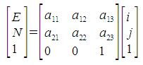
It is these six parameters (a₁₁…a₂₃)which are typically stored within a geospatial image file format to record the conversion from pixel index to geolocation. The actual conversion is described as follows:

• E = a₁₁ i + a₁₂ j + a₁₃
• N = a₂₁ i + a₂₂ j + a₂₃

where E is easting, N is northing, i is pixel column and j is pixel row. The last row of the matrix equation is always ignored, as it boils down to 1=1. It is there to make a square matrix used to calculate the inverse operation.

Link to postgis raster

The six parameters of the affine transform are given the following names in postgis raster:

• ScaleX = a₁₁
• SkewX = a₁₂
• OffsetX = a₁₃ = t_x
• SkewY = a₂₁
• ScaleY = a₂₂
• OffsetY = a₂₃ = t_y

With the exception of OffsetX and OffsetY, the names are somewhat arbitrary for the general case.