| Version 7 (modified by , 14 years ago) ( diff ) |
|---|
Coverage Concepts and PostGIS 
Introduction 
This page attempts to provide a nontechnical introduction to basic coverage concepts and relate them to various tools and items provided by PostGIS. Nearly all users of PostGIS implicitly leverage coverage concepts, whether they realize it or not. Until the advent of PostGIS raster, vector coverages were the only possible use. Now, however, PostGIS contains the building blocks for raster coverages as well. There are similarities and differences between these two types of coverages; but in order to make sense of how they are related, the concepts cannot remain implicit.
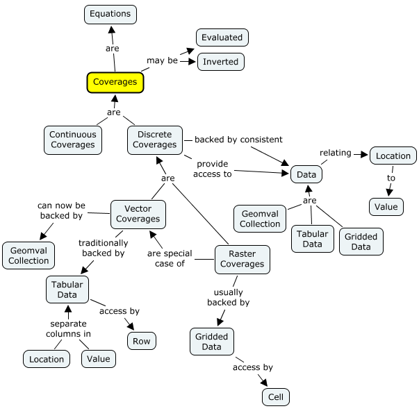
The following "concept map" gives an overview of this entire page. Starting in any box, you may read the text of the box, follow an outgoing arrow (reading the label on the way by), and read the contents of the second box. While this generally does not form complete sentences, it does provide a very visual summary of everything presented here.

Coverages are Equations 
The most fundamental thing which is true of all coverages is that they act like equations. More precisely, they act like mathematical functions. They calculate, lookup, interpolate, or return one or more values given a location and/or a time. Like mathematical functions, they may be defined everywhere (for all values) or only in certain places (e.g., only over land). The area over which a coverage is defined is the domain of that coverage. The set of values a coverage may return is the range of that coverage. This terminology is borrowed from mathematical equations.
In general, the range of a coverage is not restricted to numbers. Given a location, for instance, a "nations" coverage may return a country name which contains that location. This is a common use. The range of a coverage is not necessarily restricted to "primitive" types either: it can even return another spatial type. This will become important later. The only constraint is that a coverage has the same range (or set of potential values from which an answer may be drawn) everywhere it is defined. If it returns a "County Name" and a "Population" in one place, it returns a "County Name" and a "Population" everywhere it is defined.
Querying a coverage for a set of values given a location is called evaluating the coverage. Querying for a (set of) location(s) given some criteria on the values is given the name evaluateInverse by ISO 19123. The specifics of how answers are generated for these queries depends on the type of coverage and how the "supporting data" are stored.
As soon as you provide a way to query for an value based on a location (and optionally a time), you have created a coverage. It does not matter how the supporting data are stored, or even if supporting data even exist. The notion of a coverage is a way to define a theme or a layer which produces information without worrying about the details of how that information is produced. The coverage is the tool we use to treat vector and raster data seamlessly.
Finally, most (but not all) coverages may be inverted. Using the above example, users may ask for the set of all locations where "County Name" is "Mineral", or "Population" is 20000.
Continuous Coverages 
The easiest way to think of continuous coverages is to think of continuously varying coverages. These are coverages where every location could have a different value than its neighbors. Such a coverage may actually be implemented with an equation. Consider a "SunElevation" coverage which takes a location and a time and calculates the elevation of the sun above the horizon for that point at that time. Change either the location or the time, even slightly, and a slightly different elevation will result.
A second example of a continuous coverage is an interpolated coverage. Consider a "Temperature" coverage which is based on temperature data from a set of weather stations. The simplest way to provide approximate values in between stations is to interpolate between the nearest stations. A common way to interpolate is to use the "inverse distance weighted" (IDW) method, giving close stations more weight than far away stations. Again, if the query location is changed even a little, the answer changes too.
In PostGIS, you can implement a continuous coverage simply by writing a function which calculates a value based on location, or which interpolates the values stored in a table. Such a function is the evaluate method of a continuous coverage. If you would like your coverage to have an inverse method, you could write another function to calculate the inverse. In the case of the interpolated "Temperature" coverage above, a reasonable "inverse" method would be to allow the user to request the isotherm of a particular temperature.
Discrete Coverages 
If the easiest way to think of continuous coverages is to think of continuously varying coverages, then the easiest way to think of discrete coverages is to envision a coverage which is not continuously variable. In short: the values "jump" suddenly from one value to another. The coverage does not look "smooth" when displayed in a viewer.
Discrete coverages are not typically implemented by an equation, but are usually based on a collection of data. The collection of data is self-consistent, meaning that all data items in the collection have the same types. As the terms are commonly used, raster and vector coverages are both types of discrete coverage. They differ only in how they store and manage their collection of data. Since they are almost invariably based on a collection of data, discrete coverages offer additional functionality related to querying the data for items which match a specific criteria:
find()locates the nearest data items to a given point.select()locates all the data items within a given region.list()returns all the data items in the collection.
The most important concept of this section is that a coverage is not the same thing as the data upon which it is based. Using the same term for two different things may have been acceptable in the past, but now that raster is here, it is important to learn the difference. The differences are subtle, and it is important to master these subtleties.
Two main types of discrete coverages, in the common parlance, are "vector" and "raster". These are not distinctions present in ISO 19123, which has served as the basis of this document up to this point. We introduce the notions of vector and raster simply because the terms have a notional value, and we wish to place them in context with respect to a larger framework.
Vector Coverages 
Vector coverages are probably the most familiar type of coverage to the majority of users. The collection of data items upon which the coverage is based is usually a table. Individual data items are individual rows in the table. The columns of the table ensure that the collection is self-consistent. Each data item (row) may fill in values for each column: text may be placed in text columns, numbers in numeric columns, geometries in geometry columns, etc. The only requirement a table must fulfill in order to have the potential to supply information to a coverage is that it must have at least one geometry column and one additional column to use for a value (which may be of any type, including geometry).
The following table could serve as a collection of data items upon which a coverage could be built. Note that it has a geometry column (geom), two text columns (Name and Mayor), and two numeric columns (Elevation and Population). Each row is a data item, and each relates a point to a consistent set of values, defined by the columns. For display purposes, the "geom" column shows a point where the city belongs.

This single table could back any number of coverages. It could back a "Population" coverage simply by returning the value in the Population column whenever the query point intersects the geometry. Likewise, a coverage could return the value of any of the other columns, or any combination of the other columns. The coverage interprets the geometry column to be the domain and one or more of the other columns as the range.
Note that if there is more than one geometry column, the coverage must pick only one to use as the domain. The coverage is a way of interpreting, representing, and accessing a self-consistent collection of data.
Raster Coverages 
Raster coverages are backed by regularly gridded data. The domain is always a point. The range is one or more numeric values, referred to as "bands". Text values and timestamp values are not allowed. One can convert this gridded data into table form, if desired, although this is almost never useful. Simply construct a table with one geometry column for the cell coordinates and one numeric column for each band. Each cell in the table may then be represented by its own row. The principal advantage of the regular gridded structure is the ease with which relevant data can be located, given a spatial region of interest. This structure allows certain optimizations for speed which are not possible using a collection of data in table form.
In PostGIS, the data required to back a raster coverage is contained in a single data type called raster. This single type has both location information and value information. Each point within a raster can have it's own set of values. This subtle point has some not-so-subtle implications.
The first observation concerns the meaning of a table having a raster column. Consider a vector coverage: there is a clean one-to-one relationship between all of the values in a single row. The geometry in a particular row is associated with the values in that same row. If the geometry is a polygon, the values in the same row are associated with the entire polygon. The geometry column may contain a very complex multipolygon or a large multipoint geometry, and the value columns may be arrays, but there is no way to associate individual array elements with individual polygons or individual points. If it is necessary to associate different values with different parts of the geometry, you have to make a new row. Now consider the implications of this one-to-one relationship when one of the columns is a raster: there is still no way to associate values in other columns with individual points inside the raster. The information in the other columns applies to the entire raster.
Implication 1: A table which backs a "raster coverage" cannot be constructed by analogy with a table which backs a "vector coverage". Simply substituting
rasterforgeometryas a column type does not create data for a raster coverage. Each row in a table backing a vector coverage forms a single association between a location and a value. A row containing arasteritem contains many associations between location and value and additionally forms a single association between the raster as a whole and the rest of the values in the row.
The second observation is that each raster is self-consistent (e.g., each cell has the same number and type of bands), but there are no guarantees about how the raster in one row is related to a raster in another row (e.g., a raster in a different row may have a different number of bands, or they may be of a different type.) The column type alone is not sufficient to guarantee that all rows will have compatible data.
Implication 2: Rows of the same table cannot be assumed to convey values of consistent types. If an operation requires that values have consistent types, it may only be applied to a table which makes these guarantees: either by constraints or by carefully inserting rows from known sources.
Attachments (2)
- Cities.png (2.7 KB ) - added by 14 years ago.
- CoverageConcepts.png (68.4 KB ) - added by 14 years ago.
Download all attachments as: .zip