| Version 4 (modified by , 13 years ago) ( diff ) |
|---|
Calculating coefficients for Affine Transformation
Introduction
Geospatial rasters inherently have two coordinate systems associated with them: pixel indices and real world coordinates. Although some rasters have a very complex relationship between these two coordinate systems, many have a set of simple linear relationships between the two coordinate systems. These simple linear relationships are modular and may be combined in many ways. Regardless of the order in which they are combined, an affine transform results. The transform is then used to convert coordinates between the two coordinate systems of the raster. This page describes a set of ubiquitous individual transformations and demonstrates how they may be combined to produce an affine transformation.
The level of math required to follow along is advanced high school algebra or introductory college algebra. It should be accessible to anyone with a science, math, or engineering background. Lacking this, the nontechnical introduction to matrix multiplication on wikipedia should provide sufficient background.
Individual operations
This page discusses operations in two dimensions only. Each operation is presented as a 2x2 matrix, and each operation performs only one function. These operations were taken from wikipedia. While the matrices presented here contain the bulk of the functionality of a finished affine transform, they are not complete affine transforms themselves. Each transformation will be presented in matrix and equation form: they are equivilent representations.
Rotation
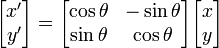
There are two directions one can rotate in two dimensions: clockwise and counter clockwise. The transformations are different. The counter-clockwise rotation is:

- x' = xcosθ − ysinθ
- y' = xsinθ + ycosθ
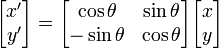
To rotate in the clockwise direction:

- x' = xcosθ + ysinθ
- y' = − xsinθ + ycosθ
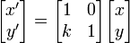
Scaling
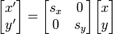
Scaling is used to set the size of the raster's grid cells in the x and y direction. The transformation is as follows:

- x' = x sx
- y' = y sy
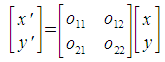
Shearing
Shearing is visually equivalent to a "slanting" which is parallel to either the x or the y axis. This is a less common operation than rotation and scaling. These are presented as individual operations: one for each axis.
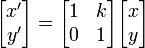
Shearing parallel to the x axis takes the following form.

- x' = x + kxy
- y' = y
While shearing parallel to the y axis has this form:

- x' = x
- y' = kyx + y
Combining individual operations
Whenever more than one of the above operations is required, they may be combined using matrix multiplication. As an example, all of the above matrices will be combined into one. The result of such a combination is still not an affine transform, however. It is just a 2x2 matrix has all the individual functions aggregated into it.
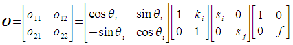
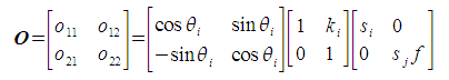
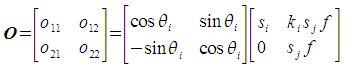
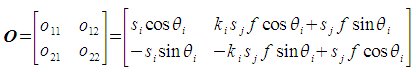
We will be calculating a new matrix, O, which is the aggregate of the following individual operations:
- scaling
- clockwise rotation
- shearing parallel to the x axis
- shearing parallel to the y axis
We do this by multiplying the 2x2 matrices of the individual operations together, as follows:

The above matrix equation is shorthand for four equations: one equation each for o11, o12, o21 and o22. We will perform the multiplications on the right hand side one at a time.
Starting from the beginning: We want to be able to calculate the parameters for an affine transform which includes the operations: scaling, translation, rotation, and skew (shearing). Matrices for these individual operations are found on http://en.wikipedia.org/wiki/Transformation_matrix#Examples_in_2D_graphics . What ho! We can combine these individual operations willy nilly by matrix multiplication. But note that these individual matrices are the only places where individual coefficients represent meaningful parameters. Once you start the multiplication, the coefficients become all jumbled up with terms combined in various ways.
So, using wikipedia plus a little customization, I've labeled the PURE coefficients (as opposed to our jumbled coefficients) as follows:
Sx : scale in the x direction Sy : scale in the y direction Tx : translation in the x direction Ty : translation in the y direction Kx : shearing parallel to x axis Ky : shearing parallel to y axis theta : angle of rotation CLOCKWISE around the origin (not around the x axis, not around the y axis: around the origin; or if you like, around the invisible Z axis coming out of the screen and poking you in the eye.)
The next step is to define an order. I chose: "Scale followed by rotation followed by shearing (skew)".
Multiplying these matrices together, as described here (http://en.wikipedia.org/wiki/Transformation_matrix#Composing_and_inverting_transformations) gives a 2x2 matrix, which is not an affine transform yet. Let's label the coefficients of this matrix as follows
| O11 O12 | | O21 O22 |
(I apologize for the ascii graphics throughout. Gmail is not using a monospaced font even in "plain text" mode.)
So what I get for these coefficients (after multiplying in the order specified) is:
O11 = Sx * (cos(theta) + Ky sin(theta)) O12 = Sx * (Kx cos(theta) + sin(theta)) O21 = Sy * (-sin(theta) + Ky cos(theta)) O22 = Sy * (-Kx * sin(theta) + cos(theta))
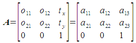
And the final bit is to add translation by making this into an affine transform:
| O11 O12 O13 | | O21 O22 O23 | | 0 0 1 |
where:
O13 = Tx O23 = Ty
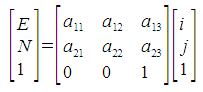
To be pedantic, this is used as follows:
| E | | O11 O12 O13 | | i | | N | = | O21 O22 O23 | | j | | 1 | | 0 0 1 | | 1 |
where: E = easting N = northing i = pixel column j = pixel row
The coefficients map onto our jumbled named coefficients as follows :
ScaleX = O11 SkewX = O12 OffsetX = O13 SkewY = O21 ScaleY = O22 OffsetY = O23
The important thing to note is that the things we're rather loosely calling Scale[XY] and Skew[XY] represent all of Scale, Rotation and Shearing. This dictates that you cannot set these coefficients without knowing all three.
Attachments (21)
- CCW_rotation.png (1.2 KB ) - added by 13 years ago.
- CW_rotation.png (1.2 KB ) - added by 13 years ago.
- scaling.png (928 bytes ) - added by 13 years ago.
- shear_x.png (867 bytes ) - added by 13 years ago.
- shear_y.png (863 bytes ) - added by 13 years ago.
- aggregate_usage.png (1.3 KB ) - added by 13 years ago.
- affinematrix.png (2.2 KB ) - added by 13 years ago.
- affineusage.png (2.1 KB ) - added by 13 years ago.
- aggregate_step1.png (3.2 KB ) - added by 13 years ago.
- aggregate_step2.png (3.0 KB ) - added by 13 years ago.
- aggregate_step3.png (2.6 KB ) - added by 13 years ago.
- aggregate_step4.odf (4.8 KB ) - added by 13 years ago.
- aggregate_step4.png (3.2 KB ) - added by 13 years ago.
- reflect_x.png (1.0 KB ) - added by 13 years ago.
- construction-step5.png (6.8 KB ) - added by 13 years ago.
- basisvector_i.png (2.4 KB ) - added by 13 years ago.
- basisvector_j.png (2.7 KB ) - added by 13 years ago.
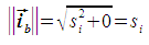
- basisvectormag_i.png (1.0 KB ) - added by 13 years ago.
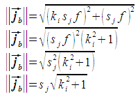
- basisvectormag_j.png (3.8 KB ) - added by 13 years ago.
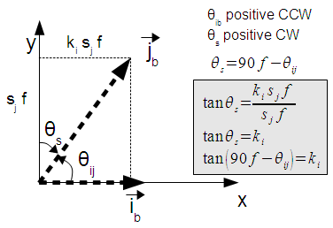
- shearing_params.png (11.4 KB ) - added by 13 years ago.
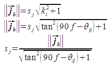
- scalefactor_j.png (3.9 KB ) - added by 13 years ago.
Download all attachments as: .zip