NAME

i.segment mean shift algorithm - Identifies segments (objects) from imagery data using mean shift algorithm.

KEYWORDS

imagery, segmentation,

SYNOPSIS

i.segment

i.segment [-dwap] group=name output=name [band_suffix=name] threshold=value [radius=value] [hr=value] [method=string] [similarity=string] [minsize=value] [memory=value] [iterations=value] [seeds=name] [bounds=name] [goodness=name] [--overwrite] [--help] [--verbose] [--quiet] [--ui]

Flags:

-d
Use 8 neighbors (3x3 neighborhood) instead of the default 4 neighbors for each pixel

-w
Weighted input, do not perform the default scaling of input raster maps

-a
Use adaptive bandwidth for mean shift
Range (spectral) bandwidth is adapted for each moving window -p
Use progressive bandwidth for mean shift
Spatial bandwidth is increased, range (spectral) bandwidth is decreased in each iteration

--o
Allow output files to overwrite existing files

--h
Print usage summary

--v
Verbose module output

--q
Quiet module output

--qq
Super quiet module output

--ui
Force launching GUI dialog

PARAMETERS

group=name [required]

Name of input imagery or imagery group

output=name [required]

Name of output segmentation map

threshold=value [required]

Difference threshold between 0 and 1 Threshold = 0 merges only identical segments; threshold = 1 merges all

band_suffix=name

Suffix for output bands with shifted mean value

radius=value

spatial bandwidth in number of cells

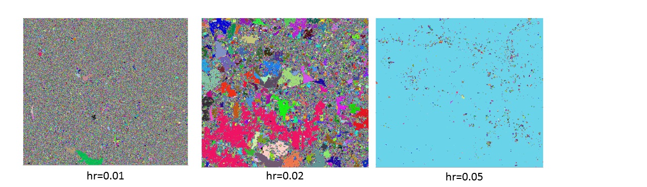
hr=value

range bandwidth in number of cells

method=string

Segmentation method Options: region_growing, mean_shift, watershed

similarity=string

Similarity calculation method Options: euclidean, manhattan Default: euclidean

minsize=value

Minimum number of cells in a segment The final step will merge small segments with their best neighbor Options: 1-100000 Default: 1

memory=value

Memory in MB Default: 300

iterations=value

Maximum number of iterations during the mean shift process

seeds=name

Name for input raster map with starting seeds

bounds=name

Name of input bounding/constraining raster map

goodness=name

Name for output goodness of fit estimate map

--overwrite

Boolean if overtie the existing raster

--ui

run with the user interface mode

--help

--verbose

--quiet

DESCRIPTION

GRASS GIS has the i.segment which provides the possibility to segment an image into objects. This is a basic step in object-based image analysis (OBIA). Currently, the module only provides one segmentation algorithm: region-growing. The code of i.segment was structured in a way that allows addition of other algorithms. It would be more useful and comprehensive to add mean-shift to the i.segment module.

Mean shift segmentation is a local homogenization technique that is very useful for damping shading or tonality differences in localized objects. For the algorithm implementation of this case, basically the algorithm replaces each pixel with the mean of the pixels in a range-r neighborhood and whose value is within a distance d. The Mean Shift usually has 3 important parameters: 1) A distance function for measuring distances between pixels. Usually the Euclidean distance, but any other well-defined distance function could be used. The Manhattan Distance is another useful choice sometimes. 2) A radius (spatial bandwidth). All pixels within this radius (measured according the above distance) will be accounted for the calculation. 3) A value difference (range bandwidth). From all pixels inside radius r, we will take only those whose values are within this difference for calculating the mean [1].

COMPARISON

Seeded Region Growing

The seeded region growing (SRG) algorithm is one of the simplest region-based segmentation methods. It performs a segmentation of an image with examine the neighboring pixels of a set of points, known as seed points, and determine whether the pixels could be classified to the cluster of seed point or not [2].
Pros:

• The image could be split progressively according to user demanded resolution because

the number of splitting level is determined by user.

• User could split the image using the criteria to be decided, such as mean or variance of segment pixel value. In addition, the merging criteria could be different to the splitting criteria

Cons:

• The blocky segment problem could be reduced by splitting in higher level, but the trade off is that the computation time will arise.

Mean shift

Numerous nonparametric clustering methods can be separated into two parts:hierarchical clustering and density estimation. Hierarchical clustering composes either aggregation or division based on some proximate measure. The concept of the density estimation-based nonparametric clustering method is that the feature space can be considered as the experiential probability density function (p.d.f.) of the represented parameter. The mean shift algorithm can be classified as density estimation. It adequately analyzes feature space to cluster them and can provide reliable solutions for many vision tasks. The basics of mean shift are discussed as below [3].

Pros:

• An extremely versatile tool for feature space analysis. Mean-shift algorithm is applicable not only in image segmentation, but also in motion detector, image filtering and etc.
• Suitable for arbitrary feature spaces.

Cons:

• The range bandwidth (hr) and spatial bandwidth (hs) are the only two factors can control the output, especially the range bandwidth results in a tremendous influence to the result.
• The computation time is quite long, for the iterations of anisotropic filtering, clustering and merging small objects.

Other segmentation methods

Watershed

The main goal of watershed segmentation algorithm is to find the “watershed lines” in an image in order to separate the distinct regions. To imagine the pixel values of an image is a 3D topographic chart, where x and y denote the coordinate of plane, and z denotes the pixel value. The algorithm starts to pour water in the topographic chart from the lowest basin to the highest peak.
Pros:

• The boundaries of each region are continuous.

Cons: The segmentation result has over-segmentation problem. The algorithm is time-consuming.

Fast scanning algorithm

The concept of fast scanning algorithm is to scan from the upper-left corner to lower-right corner of the whole image and determine if we can merge the pixel into an existed clustering. The merged criterion is based on our assigned threshold. If the difference between the pixel value and the average pixel value of the adjacent cluster is smaller than the threshold, then this pixel can be merged into the cluster.

Pros:

• The pixels of each cluster are connected and have similar pixel value, i.e. it has good shape connectivity.
• The computation time is faster than both region growing algorithm and region splitting and merging algorithm.
• The segmentation results exactly match the shape of real objects, i.e. it has good shape matching.

Hierarchical clustering

The concept of hierarchical clustering is to construct a dendrogram representing the nested grouping of patterns (for image, known as pixels) and the similarity levels at which groupings change.The hierarchical clustering can be divided into two kinds of algorithm: the hierarchical agglomerative algorithm and the hierarchical divisive algorithm.
Pros:

• The process and relationships of hierarchical clustering can just be realized by checking the dendrogram.
• The result of hierarchical clustering presents high correlation with the characteristics of original database.
• We only need to compute the distances between each pattern, instead of calculating the centroid of clusters.

Cons:

• For the reason that hierarchical clustering involves in detailed level, the fatal problem is the computation time

K-mean clustering

Pros:

• K-means algorithm is easy to implement.
• Its time complexity is O(n), where n is the number of patterns. It is faster than the hierarchical clustering.

Cons:

• The result is sensitive to the selection of the initial random centroids.
• We cannot show the clustering details as hierarchical clustering does.

NOTES

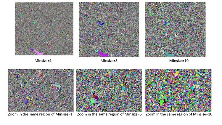
Minimum segment size

Minimum segment size is the parameter control the minimum object size interm of pixel fro the segment result. Its default value is zero while in reality the segmentation objects are always larger than 1. Considering that the result of clumping is in line with the logic of adaptive bandwidth, minimum segment size should be >1 when using adaptive bandwidth, this would connect the border cells to the appropriate segments. Such a message could be added for mean shift + adaptive bandwidth + minimum segment size = 1.

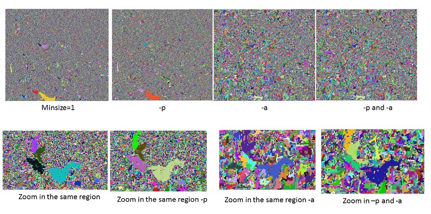
Adaptive bandwidth (-a flag)

Adaptive bandwidth means here that the range bandwidth is adapted for each moving window separately. Range bandwidth is a very important factor which control the segment result. Sometimes fixed range bandwidth in a very large region results in the over-segment or under segment in certain regions. Using adaptive bandwidth, effectively, the bandwidth becomes smaller when there focus cell differs quite a bit from its neighbors, this prevents blending of separate objects that are not clearly separated with regard to band values.

Progressive bandwidth (-p flag)

Progressive bandwidth increases the spatial bandwidth and decreases the range bandwidth with each iteration. Because the segmentation on the very large coverage involved the tremendous variabilities over the different regions, so the fixed bandwidth(s) are not suitable for the entire image. The rationale is that with each iteration, cell values are shifted a bit more towards the object's mean and become more similar to the cell's neighbors (within range bandwidth). Therefore the range bandwidth can be a bit decreased and the spatial bandwidth a bit increased. A larger spatial bandwidth means that fewer iterations are needed to shift cell values towards the object's mean.

EXAMPLES

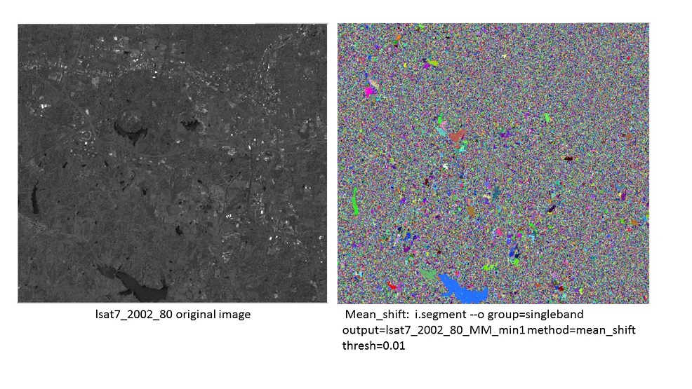
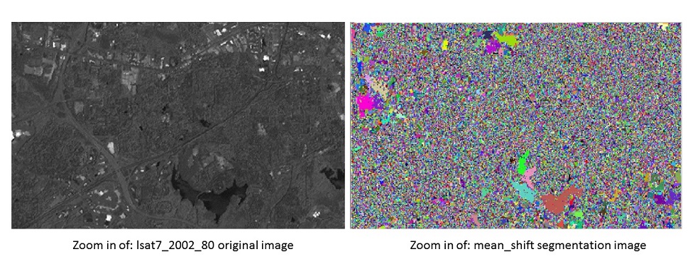
Segmentation of single band panchromatic image

This example uses the panchromatic image inluded in the NC sample dataset. Set up an imagery gourp: i.group group=singleband input=lsat7_2002_80

g.region raster=lsat7_2002_80 -p

i.segment --o group=singleband output=lsat7_2002_80_MM_min1 method=mean_shift thresh=0.01

[1] ​http://stackoverflow.com/questions/4831813/image-segmentation-using-mean-shift-explained
[2] Adams, Rolf, and Leanne Bischof. "Seeded region growing." IEEE Transactions on pattern analysis and machine intelligence 16.6 (1994): 641-647
[3] Y. Cheng, “Mean shift, mode seeking, and clustering,” IEEE Trans. Pattern Analysis and Machine Intelligence, vol. 17, no. 8, pp. 790-799, Aug. 1995
[4]Wang, Yu-Hsiang. "Tutorial: Image Segmentation." National Taiwan University, Taipei (2010): 1-36.