| Version 1 (modified by , 13 years ago) ( diff ) |
|---|
Seamless spatial operations architecture
- Seamless spatial operations architecture
- Introduction
- Scope
- Types of information
- A tour of ISO 19123
- Associations: the building blocks
- A raster is a CV_Grid
- Top level coverage
- Summary
- Representation
- Purely spatial information
- Spatial information with associated numeric value
- Summary
- Expected Results and Information types
- Result Grid Iteration Engine
- See also
Introduction
This page presents an extensible and reusable architecture capable of delivering on the promise of seamless raster and vector spatial operations. A spatial operation is any operation where the spatial characteristics of an object affect the outcome of the operation. Usually, the result of such an operation is spatial information which must somehow be conveyed.
A description of what "seamless" means, with some worked examples, may be found in the original WKT Raster presentation. This is not a well defined domain, so the architecture selected to actualize the original vision must be flexible and adaptable. It should be expected that seamless operations will evolve over time, as the facility is applied to practical problems.
Scope
This architecture articulates a strategy and best practices for developing spatial operations which evenhandedly handle raster and vector data. Common traits and requirements for such operations are expressed. This architecture assumes the ability to load, store and access raster and vector data is present, and does not include such operations.
This architecture is somewhat abstract, and while it is designed to work within the PostGIS framework (which uses the non-object-oriented language C), the fundamental concepts and structure should be applicable to any system. Implementation details are not considered here, although the structure of conforming implementations is specified.
Types of information
Vector operations operate on "vector objects", which are geometries. These geometries represent purely spatial information. Depending on the type of geometry, they may represent a single point, an array of points, lines or curves, areas, or volumes. Operations on these geometries generate purely spatial information which is also represented by a geometry (e.g., the difference between two polygons is the area of the first polygon which is not overlapped by the second one; this area is represented by a resultant polygon).
Raster operations operate on gridded data. The grid itself conveys spatial information, and the data associated with each grid cell conveys value information. Typical raster operations may operate on the spatial or the value information of a raster, or both. The result of a raster operation may also convey spatial information, value information, or both.
To handle raster and vector data seamlessly, it is first necessary to declare the types of information potentially handled by spatial operations. It is then necessary to define how each type of object may be used to communicate that information. The two categories of information addressed by this architecture are:
- Purely spatial information
- Spatial information with associated numeric value
The fundamental premise of this architecture is that there is a legitimate distinction between these types of information, but that both types of information may be conveyed using either raster or vector constructs. Operations may specify that they handle one or both types of information, and they are not required to handle the different information types evenhandedly. However, operations they should accept or produce all representations of the information they claim to handle (i.e. raster or vector.)
A tour of ISO 19123
The association of spatial information to numeric value is the fundamental building block of the coverage spatial type defined in ISO 19123. Individual associations, even aggregations of associations, are not themselves coverages. This architecture leverages the concepts developed in ISO 19123, in as far as they are applicable, in order to avoid reinventing the wheel. The intent is not to provide a conforming implementation, but to identify parallels. A complete coverage implementation may be able to leverage the building blocks defined by this architecture as a back end. With respect to the goals of this architectural definition, the principal benefit of leveraging the coverage toolbox is to aid the definition of a means to uniformly interact with fundamentally different data types.
This architecture deals only with a very limited profile of the toolbox defined in ISO 19123. Specifically, geometric objects are limited to 2 coordinate dimensions (x,y or lat,lon) and 0, 1, or 2 topological dimensions (points, lines, and polygons). In addition, the data types of associated values are constrained to numeric types (integers and floating point numbers of various sizes.) These limitations define the common ground between the capabilities of image formats (which persist raster data) and the vast majority of systems capable of handling geospatial data.
Associations: the building blocks
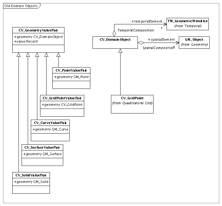
Each individual association is represented by a CV_GeometryValuePair, or one of its children. Children of CV_GeometryValuePair set limits on the spatial information allowed, and specific coverage types (e.g., point coverages) are composed of associations formed by one of these children (e.g., CV_PointValuePair). The hierarchy is given in the following figure.
This architecture does not require a full implementation of the entire hierarchy. Only two data types are required: CV_GeometryValuePair and CV_GridPointValuePair. The names of the implementing data types are unimportant, they must simply occupy the roles in the above diagram. Rigid adherence to the UML diagram would require that a CV_DomainObject be explicitly represented. This architecture specification allows the direct substitution of a geometry object for the cases where a temporal component is not part of the domain. If the domain is to include temporal information, however, a domain object with both a spatial and temporal component must be defined.
The "value" field of the CV_GeometryValuePair must be constrained to be a list of numeric types (each member of the list may have different types). Alternatively, a data structure type, such as "struct" in C, may be used, provided that all the fields are numeric. When applied to a raster, the "value" field represents the information in all the raster's bands (or a subset thereof), in order.
A raster is a CV_Grid
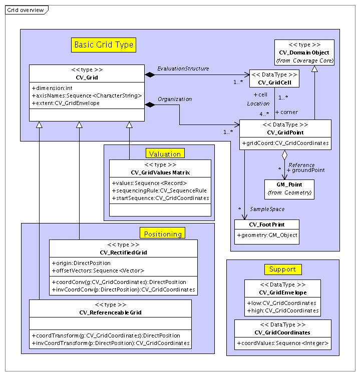
A raster is more than a single association of spatial information to value information, yet less than a coverage. The raster data type is an aggregation of many individual associations which possess a gridded spatial structure. A georeferenced raster ties this gridded spatial structure to geolocations. A raster is, in short, a means of efficiently representing many values which are associated with many places. The following UML diagram shows the relevant constructs defined by ISO 19123.
A CV_Grid by itself consists only of the metadata necessary to define a regular grid: number of dimensions, extent along each axis, and names for the axes. This constitutes basic header metadata only. There is no geospatial information at all. The data are also absent. All instances of CV_Grid may be related to certain other basic structures, as shown in the figure. However, the meaning of these structures and the extent to which they are populated with information, may vary depending on the information available.
Children of CV_Grid add functionality. Children in the "Positioning" box add georeferencing information and capabilities. Children in the "Valuation" box add the raster data itself, as well as the ability to access it. Each child in the "Positioning" box represents a type of geolocation, adding the ability to translate back and forth between grid indices and location on the ground. This is equivilent to loading a header with geotags which specify the projection type as well as supplying all the parameters necessary to calculate position. An instance of a child in the "Valuation" box understands how to access the data, whether in memory or in a file. For the purposes of this architecture specification, a raster is the union of a member in the Positioning box with a member of the Valuation box: representing a fully georeferenced grid type with full access to the gridded data (whether that data is on disk or in memory).
The CV_GridPoint, articulated in the above figure, differs from a CV_DomainObject only in the ability to store the grid coordinates as well as the geolocation. This is not considered critical. The associations with other pieces of information (such as CV_Footprint or CV_GridCell) need not be explicitly maintained so long as they can be calculated. This architecture specification does not require the explicit implementation of a separate CV_GridPoint type. In fact, a loose interpretation of ISO 19123 is encouraged in this case, particularly due to the fact that raster cells may be interpreted as points or as cell areas. It is explicitly considered permissible to construct an association between the polygon forming the outline of the grid cell and the cell's values (as a CV_GeometryValuePair), instead of using the prescribed CV_GridPointValuePair. If it is necessary to represent the gridded data using these individual associations, the spatial object should accurately reflect the point or area to which the values apply.
It is rarely necessary or desirable to represent a raster as a collection of CV_GeometryValuePairs, however it is useful to explicitly articulate the fact that the raster is composed of these individual associations. It is also useful to explicitly acknowledge that each grid point has a footprint, and each grid cell is bounded by four grid points (again, loosely interpreting this to mean that grid points may constitute the center of four grid cells instead of the four corners of a single cell.) Calculating the footprint of an individual cell may be a useful utility to include in a software package. Internally representing the gridded data in this structure is generally not necessary because the spatial location is generally trivial to compute on the fly.
Top level coverage
The basic top level schema for the coverage type is defined in the figure below. This builds on the tools provided previously and provides a common access mechanism which does not depend on the type of the underlying data.
Coverages add value over a simple collection of geometry-value pairs. They ensure that the collection of geometry-value pairs has a consistent value (e.g., values in the coverage have the same "type" everywhere). Three methods (find, select, and list) are shown on the Coverage type itself. Another method, an important method, is not shown on this diagram: evaluate.
| Method | Description |
evaluate |
returns a set of values for a given point. |
select |
returns all the geometry-value pairs which "lie within" the provided geometry |
find |
returns a list of geometry-value pairs, in order of distance from the provided point |
list |
returns a list of all the constituent geometry-value pairs which make up the coverage |
evaluateInverse |
returns a set of locations which match a particular set of values |
These methods are the same for all coverages, regardless of type. The two main children of a CV_Coverage create a distinction between discrete coverages, which are simple aggregations of individual geometry-value pairs; and continuous coverages, which are capable of interpolating between geometry-value pairs. Both types of coverages are defined by geometry-value pairs.
Summary
ISO 19123 provides tools to handle the association of a spatial object with a value. It defines a mechanism to accomplish this association which is conceptually similar regardless of the geometric objects participating in the association. It explicitly articulates how gridded information may be expressed as a set of these associations. Tools provided by ISO 19123 outline the seamless treatment of raster and vector data as two alternate expressions of the same information.
Representation
This architecture considers "raster" and "vector" data types to be representational tools. Each representational tool is a means of conveying information. Each has different expressive capabilities. In addition, two distinct types of information have been articulated. These are: purely spatial information; and spatial information having an associated numeric value. This architecture defines a means to represent each information type using each representational tool.
Purely spatial information
Vectors represent purely spatial information using geometry objects. These may be arbitrarily complex, and the constituent points are not necessarily aligned to any particular grid.
Rasters represent purely spatial information using a mask. A mask is a special case of a raster where the grid cells hold true or false values. Each grid cell possesses spatial location information (e.g., for each grid cell (i, j), a real-world position can be calculated). A true value in a cell indicates that the spatial location associated with the cell is included in the spatial information conveyed by the raster. Likewise, a false value indicates that the spatial information associated with the cell is not included. The spatial information conveyed by the raster as a whole is the sum of its parts. More specifically, the spatial information conveyed by the overall raster is the union of the spatial information conveyed by each cell with a true value.
Spatial information with associated numeric value
Vectors represent combined spatial and value information with a structure, record, datatype, or class which has a geometry part and a value part. In ISO 19123 this is represented as the type CV_GeometryValuePair. In the postgis raster extension, there is a geomval type. Any data structure which enforces a one-to-one relationship between a particular geometry and a particular list of values will accomplish this end. Using such a structure, there is a clear separation: the geometry conveys the spatial information and the value conveys the value information.
Rasters have the ability to store one or more numeric values at each cell. The number of values present at each cell is exactly equal to the number of bands present in the overall raster. Each band may have a different numeric type, and the bands are ordered. Spatial information is conveyed by "nodata" values: cells containing the "nodata" value are equivalent to cells in a mask containing "false" values. Conversely, cells containing any value other than the "nodata" value are equivalent to cells in a mask containing true values. Each band may possess a unique "nodata" value which applies only to that band.
Rasters have the potential to specify different spatial information with each band, whereas vectors may specify only one. In order to treat vectors and rasters uniformly, this architecture requires that all bands of a raster convey the same spatial information. All bands for a given grid cell must contain the "nodata" value, or all bands for a given grid cell must contain a value other than "nodata". This architecture forbids a raster to contain grid cells where some bands are nodata and others are not.
Vectors have the potential to specify values other than numbers. This is beyond the capability of rasters, and therefore the structure which associates a geometry with a list of values must limit the list of values to numeric types. The list of values is ordered, and the type of each element in the list may be different, just as the bands of a raster may have different types.
Summary
Using these conventions, both vectors and rasters may represent spatial information associated with a value. Likewise, both vectors and rasters may represent purely spatial information. Once the type of information is known, the method to represent the information is straightforward.
Expected Results and Information types
The following table lists the potential combinations of inputs and output for two-input spatial operations. Implementations of spatial operations may declare that they support one or more rows from this table.
| Combination | Input 1 | Input 2 | Returns |
| 1 | Pure Spatial | Pure Spatial | Pure Spatial |
| 2 | Pure Spatial | Spatial+Value | Pure Spatial |
| 3 | Spatial+Value | Pure Spatial | Pure Spatial |
| 4 | Spatial+Value | Spatial+Value | Pure Spatial |
| 5 | Pure Spatial | Pure Spatial | Spatial+Value |
| 6 | Pure Spatial | Spatial+Value | Spatial+Value |
| 7 | Spatial+Value | Pure Spatial | Spatial+Value |
| 8 | Spatial+Value | Spatial+Value | Spatial+Value |
A "Pure Spatial" information type may be represented by either a geometry or by a mask (a special case of the raster data type). The Spatial+Value information type may be represented by either a non-mask raster, or by a datatype which implements the CV_GeometryValuePair from ISO 19123. The following table describes the mapping between information types and data types.
| Pure Spatial | Spatial+Value | |
| Vector | CV_DomainObject or GM_Object |
CV_GeometryValuePair |
| Raster | CV_Grid (mask) |
CV_Grid (values) |
Note that the same data type (an implementation of CV_Grid from ISO 19123) is capable of communicating both Pure Spatial and Spatial+Value information for "Raster" data. The difference is in the values of the grid cells, not in the type of the data. This reduces the number of required data types from four to three. CV_Grid will be referred to as raster, GM_Object will be referred to as "geometry", and CV_GeometryValuePair will be referred to as "geomval".
Example 1: Consider the intersection operation: returning common area between two inputs. The vector support in GIS systems is typically one eighth of the row which specifies that two Pure Spatial inputs result in a Pure Spatial output (combination 1). Typical GIS systems implement one eighth of this row due to the fact that they typically operate only on (and only return) geometry objects. A system implementing seamless vector and raster operations would also provide a means to return a mask, which is a special type of raster. Therefore, in terms of data types, this one line would become the following table. Note that because we are expanding the "Purely Spatial" line in the information type table, all of the rasters are actually masks: they lack value information. Observe also that adding the ability to return as well as accept spatial information using either representation adds support for the last seven lines of the data type table.
Input 1 Input 2 Returns geometry geometry geometry geometry raster geometry raster geometry geometry raster raster geometry geometry geometry raster geometry raster raster raster geometry raster raster raster raster
Example 2: Consider an intersection operation returning values from one of the inputs in the common area. This is sometimes known as a "clip" operation. In typical GIS systems, this is usually implemented as an operation which accepts a raster and a vector, returning a raster. In a seamless raster/vector system, the same operation is defined in terms of information type. To be as similar as possible to the traditional GIS implementation would require that the seamless operation support only lines with one Purely Spatial input and one Spatial+Value input, returning a Spatial+Value result (combinations 6 and 7). To be fully seamless, all variants of the operation listed in the data type table should be implemented. There may be a justification for intentionally supporting a less than fully seamless operation. In this case, implementers may decide to support only those variants which return a raster, as the expected result of a "clip" operation is a grid which only contains values over the spatial intersection of two objects. Alternatively, the same operation having a different return type (or taking different arguments) may be known by different names. These aspects must be considered individually for each operation as they are defined.
Input 1 Input 2 Returns Comment geometry raster raster input 2 must contain values raster geometry raster input 1 must contain values raster raster raster one input must contain values and the other must not geomval raster raster input 2 must be a mask raster geomval raster input 1 must be a mask geometry geomval raster geomval geometry raster geometry raster geomval input 2 must contain values raster geometry geomval input 1 must contain values raster raster geomval one input must contain values and the other must not geomval raster geomval input 2 must be a mask raster geomval geomval input 1 must be a mask geometry geomval geomval geomval geometry geomval
Result Grid Iteration Engine
One tool with the potential to greatly aid the implementation of any spatial operation which returns a raster is a generic engine which iterates over the result grid. Such a tool will only aid those variants which return a raster (either a mask or a value-containing raster). This tool is strictly an evaluation engine, which iterates over a provided grid to determine which cells are included in (or excluded from) the result, and which produces a value for every cell in the grid.
Ideally, the iteration engine itself should not care about the information type of the inputs. For each output raster cell, a two input engine needs to determine:
- Spatial information
- Does "Input 1" contain (or intersect) the output cell?
- Does "Input 2" contain (or intersect) the output cell?
- Is the output cell included in the result?
- Value information
- Is "Input 1" Spatial Only or Spatial+Value?
- If Spatial+Value and "Input 1" contains the output cell, what is the value?
- Is "Input 2" Spatial Only or Spatial+Value?
- If Spatial+Value and "Input 2" contains the output cell, what is the value?
- Given spatial information, and potentially value information, for "Input 1" and "Input 2", what is the value to store in the result cell?
- Is "Input 1" Spatial Only or Spatial+Value?
These determinations can be factored out of the main iteration engine as "extension points". Potential extension points may be defined as follows:
- Input
- Does input contain a point?
- Is input spatial only or Spatial+Value?
- What is the value of input at the specified point?
- Spatial operation (is the output cell included in the result?)
- Value computation (what is the value to store in the result?)
A very generic core utility could be provided with the definition of:
- Input extension points defined for
geometry,geomval, andrasterdata types. - Spatial operation extension points defined for common operations: difference, intersection, symmetric difference, and union.
- Value computation extension points defined for: mask value, copy value from input 1 (preferred) or input 2 (if necessary), expression evaluation.
Such a core utility would be called with different arguments in order to handle different combinations of input arguments, spatial operations, and value computations. Each extension point represents a well-encapsulated, reusable module which can be combined in many ways with other extension points. There is only one grid iteration engine (for the two input case), and it contains only the basic iteration logic; as the logic for other necessary pieces has been factored out to separate modules.
See also
- Original WKT Raster presentation (now Postgis Raster)
- Postgis Raster Home Page
- ISO 19123 Primer
Attachments (7)
-
coverage.png
(18.4 KB
) - added by 13 years ago.
top level coverage schema
-
grid.png
(16.9 KB
) - added by 13 years ago.
UML of CV_Grid schema
-
orig-gvp.png
(9.7 KB
) - added by 13 years ago.
UML of CV_GeometryValuePair and friends
-
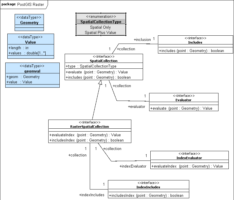
spatialcollection.png
(15.2 KB
) - added by 13 years ago.
UML Diagram of spatial collection type
- singlecollection.png (7.6 KB ) - added by 13 years ago.
- twoelementcollections.png (6.9 KB ) - added by 13 years ago.
- twoelementimplementation.png (7.8 KB ) - added by 13 years ago.
Download all attachments as: .zip