Calculating coefficients for Affine Transformation

Introduction

Geospatial rasters inherently have two coordinate systems associated with them: pixel indices and real world coordinates. Although some rasters have a very complex relationship between these two coordinate systems, many have a set of simple linear relationships between the two coordinate systems. These simple linear relationships are modular and may be combined in many ways. Regardless of the order in which they are combined, an affine transform results. The transform is then used to convert coordinates between the two coordinate systems of the raster. This page describes a set of ubiquitous individual transformations and demonstrates how they may be combined to produce an affine transformation.

The level of math required to follow along is advanced high school algebra or introductory college algebra. It should be accessible to anyone with a science, math, or engineering background. Lacking this, the nontechnical introduction to ​matrix multiplication on wikipedia should provide sufficient background.

Individual operations

This page discusses operations in two dimensions only. Each operation is presented as a 2x2 matrix, and each operation performs only one function. These operations were taken from ​wikipedia. While the matrices presented here contain the bulk of the functionality of a finished affine transform, they are not complete affine transforms themselves. Each transformation will be presented in matrix and equation form: they are equivilent representations.

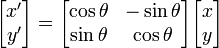
Rotation

There are two directions one can rotate in two dimensions: clockwise and counter clockwise. The transformations are different. The counter-clockwise rotation is:

• x' = xcosθ − ysinθ
• y' = xsinθ + ycosθ

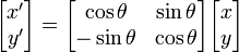
To rotate in the clockwise direction:

• x' = xcosθ + ysinθ
• y' = − xsinθ + ycosθ

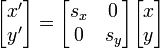
Scaling

Scaling is used to set the size of the raster's grid cells in the x and y direction. The transformation is as follows:

• x' = x s_x
• y' = y s_y

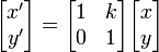
Shearing

Shearing is visually equivalent to a "slanting" which is parallel to either the x or the y axis. This is a less common operation than rotation and scaling. These are presented as individual operations: one for each axis.

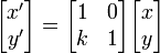
Shearing parallel to the x axis takes the following form.

• x' = x + k_xy
• y' = y

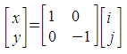
While shearing parallel to the y axis has this form:

• x' = x
• y' = k_yx + y

Combining individual operations

Whenever more than one of the above operations is required, they may be combined using ​matrix multiplication. As an example, all of the above matrices will be combined into one. The result of such a combination is still not an affine transform, however. It is just a 2x2 matrix has all the individual functions aggregated into it.

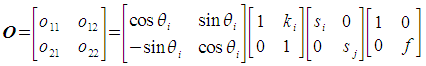
We will be calculating a new matrix, O, which is the aggregate of the following individual operations:

1. scaling
2. clockwise rotation around the origin
3. shearing parallel to the x axis
4. shearing parallel to the y axis

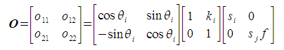
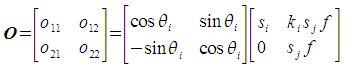
We do this by multiplying the 2x2 matrices of the individual operations together, as follows:

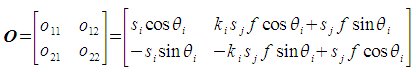
The above matrix equation is shorthand for four equations: one equation each for o₁₁, o₁₂, o₂₁ and o₂₂. We will perform the multiplications on the right hand side one at a time.

• o₁₁ = s_x ( (1 + k_x k_y) cosθ + k_y sinθ )
• o₁₂ = s_x ( k_x cosθ + sinθ )
• o₂₁ = s_y ( -(1 + k_x k_y) sinθ + k_y cosθ )
• o₂₂ = s_y ( - k_x sinθ + cosθ )

Notice that none of the coefficients in the O matrix may be said to represent pure scaling, rotation or shearing. Rather, they all have components of each of these operations factored in. If a particular transformation is not needed (say there is no shearing in either the x or y directions), then the relevant parameters may be set to zero (k_x = k_y = 0).

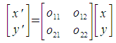
Also notice that it is not necessary to compute this matrix every time one wants to convert between pixel indices and geographic location. The coefficients are computed once for the entire raster, and may be reused for every pixel calculation. You would use this aggregate matrix O exactly as you would use any of the individual matrices:

• x' = o₁₁ x + o₁₂ y
• y' = o₂₁ x + o₂₂ y

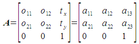
Constructing the affine transformation

The 2x2 matrix O is the upper-left hand corner of the affine transformation, which is the 3x3 matrix, A. The right hand column contains the offsets, or translation, of the raster in the x and y directions. The bottom row is always filled with the numbers 0, 0, 1. The result of this is that there are six parameters to an affine transformation which can actually change, as shown:

• a₁₁ = o₁₁ = s_x ( (1 + k_x k_y) cosθ + k_y sinθ )
• a₁₂ = o₁₂ = s_x ( k_x cosθ + sinθ )
• a₁₃ = t_x
• a₂₁ = o₂₁ = s_y ( -(1 + k_x k_y) sinθ + k_y cosθ )
• a₂₂ = o₂₂ = s_y ( - k_x sinθ + cosθ )
• a₂₃ = t_y

where:

• s_x : scale factor in x direction
• s_y : scale factor in y direction
• t_x : offset in x direction
• t_y : offset in y direction
• θ : angle of rotation clockwise around origin
• k_x : shearing parallel to x axis
• k_y : shearing parallel to y axis

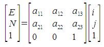
It is these six parameters (a₁₁…a₂₃)which are typically stored within a geospatial image file format to record the conversion from pixel index to geolocation. The actual conversion is described as follows:

• E = a₁₁ i + a₁₂ j + a₁₃
• N = a₂₁ i + a₂₂ j + a₂₃

where E is easting, N is northing, i is pixel column and j is pixel row. The last row of the matrix equation is always ignored, as it boils down to 1=1. It is there to make a square matrix used to calculate the inverse operation.

Link to postgis raster

The six parameters of the affine transform are given the following names in postgis raster:

• ScaleX = a₁₁
• SkewX = a₁₂
• OffsetX = a₁₃ = t_x
• SkewY = a₂₁
• ScaleY = a₂₂
• OffsetY = a₂₃ = t_y

With the exception of OffsetX and OffsetY, the names are somewhat arbitrary for the general case.